Introducing gismo: a tool for finding grouped independent supports

My first paper since joining Prof. Dr. Kuldeep Meel’s group at the National University of Singapore (NUS) has been accepted to IJCAI 2023! The topic of this paper was a completely new direction for me, and I learned a lot during this project. I had the great privilege to work with Kuldeep and with Prof. Dr. Arunabha Sen for Arizona State University (ASU) on this project, and learned a lot from each of them. In this blog post, I will share a bit about the problem that we solve, why it needs solving, and how we solve it, introducing our new tool: gismo.

Note: this blog post was written to give intuitions and provide more figures and tables to help understand the material. For a more formal description, please click here to go to a page with links to the paper, the extended version of the paper, our code, slides, a poster, a short video, and our .bib file.

Exchanging space for time?

As each constraint programmer knows, the way that you choose to model your problem is at least as important as the way you choose to solve it. However, no matter how good your favourite encoding is, you will inevitably stumble upon a problem whose encoding size is so large, that you cannot store it in your RAM.

If you do not want to give up on your favourite encoding, you will have to give up on the solver that you are using, instead. Maybe you can come up with a streaming algorithm for your problem? Maybe you can let go of some theoretical guarantees?

We wondered what we could achieve by changing the encoding. What if we could come up with an exponentially more succinct encoding than that of the current state of the art? What would we have to give up on, then? Maybe we can gain an exponential reduction in size in exchange for higher theoretical complexity? If so, can we design a solver for that harder problem that is fast in practice? If so, can we use that solver to solve exponentially larger problem instances than the current state of the art?

In this work, we present a case study of an NP-hard problem, the generalised identifying code set (GICS) problem¹, which we reduce to a computationally harder problem: that of finding a grouped independent support (GIS) of a Boolean formula (more on that later). We then design and implement a new solver, gismo, for finding the grouped independent support of a Boolean formula, and demonstrate how effective gismo is in solving the GICS problem.

Hotel fire safety

Let me explain the generalised identifying code set (GICS)¹ problem with an example.

A famous hotel

I am known among my coworkers as someone who gets a bit agitated about fire safety².

Right now, I live in Singapore, which is famous for many things, including the impressive Marina Bay Sands hotel (MBS):

The famous Marina Bay Sands hotel, with the ArtScience museum on the left, and the symbol of Singapore, the Merlion, in the foreground on the right. Photo by: Anna Latour

The dynamics of smoke detection

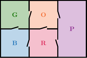
With its 2600 rooms, organised into three 57-story towers, MBS is a little too big for us to use as a toy example, so let’s just use a cosy, imaginary hotel with only 5 rooms, instead:

We imagine that we can place smoke detectors in the rooms. For example, we could place a smoke detector in the blue room, and one in the orange room:

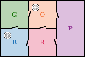
These smoke detectors have the property that they can detect smoke from a fire in the same room as they were placed in immediately, but can detect smoke from a fire in an adjacent room with a small time delay. We assume that fires do not have time to spread, and that smoke detectors cannot sense smoke further than one room away.

We imagine that the hotel’s concierge has a dashboard with an indicator light for each smoke detector. Hence, if a fire breaks out in the blue room at time $t_0$, the detector in the blue room immediately detects the smoke, and the indicator light for that detector turns blue at time $t_0$. We assume that a light stays on until we turn it off, so at time $t_1 = t_0 + 1$, the blue light is still on. Here is an example of the pattern that we see when there is a fire in the green room:

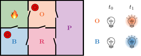
A unique signature

The pattern that we see above when there is a fire in the green room, is that at $t_0$, when the fire breaks out, none of the detectors detect any smoke. Hence, all lights are off. At time $t_1$, however, the smoke has travelled from the green room to the blue and orange rooms, so the detectors in those rooms detect the smoke, and their corresponding lights on the indicator dashboard turn on. Hence, at time $t_1$, both the blue and the orange light are on.

We call a pattern like this a signature³. Ideally, each room should have a unique signature, so we know where to send the firefighters when a fire breaks out. Looking at the figure above, you have probably realised that in this case, we cannot distinguish a fire in the green room from a fire in the red room, because they would both have the same signature.

The GICS problem asks to find out in which rooms we should place a smoke detector, such that all fires are detected, and uniquely identified. The goal is to minimise the number of smoke detectors that we place.

A graph as a model

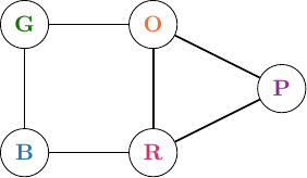
Let us make this a bit more abstract. In particular: let us model the hotel as a graph $\Gamma := (V, E)$. Each node in $V$ represents a room, and there is an edge between two nodes if their corresponding rooms are adjacent:

The GICS problem asks to find a dominating set with specific properties. We will call this set $D$, and it will correspond to the set of rooms in which we place a smoke detector. $D$ is called a generalised identifying code set of a graph $\Gamma := (V,E)$ if each node has a unique signature. The goal is to minimise the cardinality of $D$.

We will model the signatures of the nodes as tuples of sets of nodes: $\sigma_{v} := \langle S_v^0, S_v^1 \rangle$. Here, the first element of the signature, $S_v^0 := \{v\} \cap D$, models the indicator lights that are on at $t_0$ if a fire breaks out in room $v$ at time $t_0$. The second element of the signature, $S_v^1 := N_1^+(v) \cap D$, models the indicator lights that are on at $t_1$. Here, $N_1^+(v) := N_1(v) \cup \{v\}$ is the closed 1-neighbourhood of node $v$.

A solution?

Now, let’s check if our candidate solution, $D := \{B, O\}$ is indeed a solution to the GICS problem on this graph. We can simply write down all the signatures:

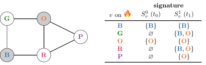
Unsurprisingly, we conclude that this $D$ is no solution to our problem. We can add a smoke detector to the purple room, however, and see what happens:

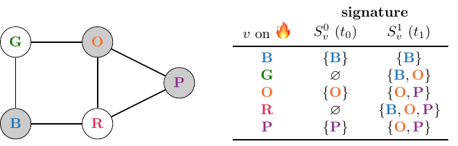
Now, we see that each fire can be uniquely identified. However, the problem was also to minimise the cardinality of $D$. In this case, we can do that by removing the smoke detector from the orange room:

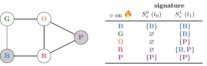
A generalisation

In the context of detecting fires in a hotel, it is not unreasonable to assume that there is only ever one fire breaking out at a time. However, other applications of identifying codes include detecting criminals in social networks (Basu & Sen, 2021a), and detecting spreaders of misinformation in online networks (Basu & Sen, 2021b). In those contexts, it is reasonable to assume that more than one ‘fault’ occurs in the network at the same time.

We denote the maximum number of simultaneous faults with $k$, and it reflects the maximum number of nodes that can reasonably be expected to ‘fail’ at the same time. In our example: it is the maximum number of rooms that can catch fire at the same time.

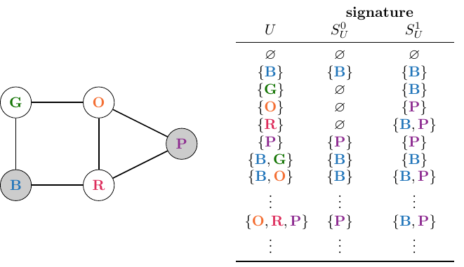
In the example above, we had implicitly assumed that $k = 1$. However, we could generalise the concept of closed 1-neighbourhoods and signatures to be defined for sets of nodes rather than individual nodes. In particular, we can define $N_1^+(U) := \bigcup_{v \in U} N_1^+(v)$ as the closed 1-neighbourhood of set of nodes $U \in V$, and update the definition of the signature accordingly: $\sigma_U := \langle S_U^0, S_U^1\rangle$, with $S_U^0 := U \cap D$ and $S_U^1 := N_1^+(U) \cap D$.

We update the table of signatures accordingly:

Hence, the problem that we study in this work is as follows:

Given a network $\Gamma := (V,E)$ and a maximum number of simultaneous failures $k$, find a dominating set $D \subseteq V$ such that for each pair of sets $U, W \subseteq V$, it holds that $\sigma_U \neq \sigma_W$, and $| D|$ is minimised.

Current state of the art

The approach taken by the current state of the art is to encode this NP-hard problem as an integer-linear program (ILP), and to use an off-the-shelf MIP solver like CPLEX to solve it. The problem with this approach is that it does not scale well with the number of nodes in the network $V$ and the maximum number of simultaneous failures $k$.

Intuitively, this approach explicitly encodes that all pairs of rows in the table above have to be different from each other. As a result, the number of linear constraints in the encoding scales exponentially with $k$. Hence, the ILP encoding of the GICS problem has $O(\binom{|V|}{k}^2)$ linear constraints, which grows as $O(|V|^k)$, and hence is exponential in $k$. In this work, we adapted the encoding from (Padhee, Biswas, Pal, Basu and Sen, 2020) to work for $k > 1$.

In this work, we propose to reduce the GICS problem to the computationally harder problem of finding a grouped independent support of a Boolean formula, which I will say a bit more about now.

Background: Independent supports

Let’s first get an intuition for what an independent support is, and then define the concept of a grouped independent support.

Independent Support

Intuitively, the independent support $I$ of a Boolean formula $F(X)$ (Chakraborty, Fremont, Meel, Seshia and Vardi, 2014) is a subset of variables with the special property that for all solution of $F(X)$, the truth values of the variables in $I$ uniquely determine the truth values of the variables in $X - I$. I will illustrate this with an example.

Consider the following Boolean formula on three variables: $F(X) := (x_1 \lor x_2) \leftrightarrow x_3$. Here is a truth table for this formula, which only lists the variable assignments that are solutions to this formula (here, I am using $\sigma: X \mapsto {0,1}$ to indicate an assignment of truth values to variables, rather than a signature of a (set of) node(s)):

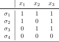
Let us now look at two different ways of projecting these solutions on subsets of variables:

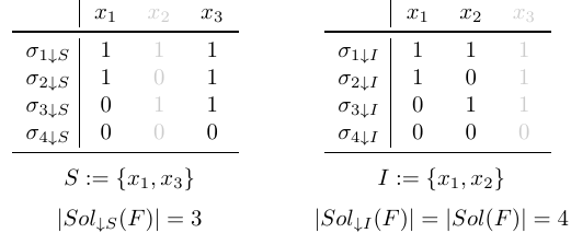
In the left table, we see that projected solutions $\sigma_{1 \downarrow S}$ and $\sigma_{2 \downarrow S}$ coincide, e.g., $\sigma_{1 \downarrow S} = \sigma_{2 \downarrow S}$. Hence, the cardinality of the set of projected solutions is smaller than the cardinality of the set of full solutions. On the other hand, in the right table, we see that none of the projected solutions coincide: all projected solutions are unique. Hence, projecting on projection set $I := \{x_1, x_2\}$ preserves the cardinality of the set of solutions in this example.

This is another way to look at independent supports of Boolean formulae. An independent support $I \subseteq X$ of a Boolean formula $F(X)$ is a subset of variables that preserves the cardinality of the set of solutions under projection. We will use this property later on, in our reduction of the generalised identifying code set problem to the grouped independent support problem.

Grouped Independent Support (GIS)

In our work, we define a grouped independent support (GIS) as an extension of the vanilla independent support. We assume that we are given not only Boolean formula $F(X)$, but also a partition of $X$, $\mathcal{G}$. We now ask to find a subset of that partition $\mathcal{I} \subseteq \mathcal{G}$ such that $I := \bigcup_{G \in \mathcal{I}} G$ is an independent support of $F(X)$. Now, variables are grouped together in little subsets of variables. A variable can only be added to an independent support together with all variables in its group. Hence, for each group, it holds that either all variables in that group end up in the GIS, or none of them do.

Let’s consider an example, for the same example Boolean formula as above, $F(X) := (x_1 \lor x_2) \leftrightarrow x_3$. Consider the partition $\mathcal{G}_1 := \{\{x_1, x_2\}, \{ x_3 \}\}$. Since $I := \{x_1, x_2\}$ is an independent support of $F(X)$, a grouped independent support of $\langle F(X), \mathcal{G}_1 \rangle$ is $\mathcal{I}_1 := \{\{x_1, x_2\}\}$.

Now consider the following partition: $\mathcal{G}_2 := \{\{x_1\}, \{x_2, x_3\}\}$, instead. Now, since neither $\{x_1\}$, nor $\{x_2, x_3\}$ is an independent support of $F(X)$, the only possible grouped independent support that we can find for $\langle F(X), \mathcal{G}_2 \rangle$, is $\mathcal{I}_2 = \mathcal{G}_2 = \{\{x_1\}, \{x_2, x_3\}\}$, since $\{x_1, x_2, x_3\} = X$ is an independent support of $F(X)$.

We now define the GIS problem as follows:

Give a Boolean formula $F(X)$ and a partition of the variables $\mathcal{G}$, find a subset $\mathcal{I} \subseteq \mathcal{G}$ such that $I := \bigcup_{G \in \mathcal{I}} G$ is an independent support of $F(X)$, and $| \mathcal{I} |$ is minimised.

Reduction

So how do we reduce the GICS problem to the GIS problem? That’s a great question, I’d love to tell you!⁴

The Boolean Formula

As mentioned above, GICS problems are typically formulated on graphs. Given a graph $\Gamma := (V,E)$, we define two variables for each node $v \in V$. One variable, $x_v$, models the first element of the signatures. The other variable, $y_v$, models the second element. We partition the set of all variables as follows: $\mathcal{G} := \{ G_v := \{x_v, y_v\} \mid v \in V\}$. Hence, in the hotel example problem above, we would have ten variables, partitioned into five groups.

Key to our reduction is that we assume that each room has a smoke detector, and then remove smoke detectors from rooms, until we have the smallest possible set of rooms with smoke detectors, such that each set of fires of cardinality at most $k$ can be uniquely identified.

Assuming that each room contains a smoke detector, variable $x_v$ is an indicator variable that is True if the smoke detector in room $v$ detects smoke at time $t_0$. Note that this means that $x_v$ is essentially an indicator variable that is True if a fire breaks out in room $v$ at $t_0$, and False otherwise. Similarly, $y_v$ is an indicator variable that is True if the smoke detector in room $v$ detects smoke at time $t_1$.

Recall the dynamics of smoke detectors detecting smoke from the same room and from adjacent rooms. We can model these dynamics in the following set of constraints:

We must also encode the assumption that at most $k$ fires break out at the same time, and do that with a cardinality constraint:

Hence, we obtain the following formula:

Note that we need $| V | + \sum_{v \in V} deg(v) = 2 \cdot | E | + | V | = O(| E |)$ material equivalences to encode $F_{\text{detection}}$, and that $F_{\text{cardinality},k}$ can be encoded using $O(k \cdot | V |)$ clauses (Sinz, 2005).⁵ Hence, in this encoding, $F_k (X,Y)$ has $O(k \cdot | V | + | E |)$ clauses. Note that our encoding grows linearly with both network size and $k$, whereas the ILP encoding of the former state of the art grows exponentially with $k$.

The Solution to the GICS Problem

By construction, the above formula has exactly 1 solution for each signature that we need. After all, $F_{\text{detection}}$ is always satisfiable without any additional constraints. However, adding $F_{\text{cardinality},k}$ ensures that the only solutions are those in which at most $k$ variables in $X$ are True, while the others are False. Hence, we have $\sum_{j=0}^k \binom{| V |}{k}$ solutions to $F_k (X,Y)$.

The trick is to find a GIS $\mathcal{I} \subseteq \mathcal{G}$, such that when we project all solutions to $F_k (X,Y)$ on $I := \bigcup_{G \in \mathcal{I}} G$, we preserve the cardinality of the set of projected solutions, and minimise the cardinality of $\mathcal{I}$. Now, each group in $\mathcal{I}$ corresponds to exactly one node, such that the solution to the GICS problem is $D := \{ v \in V \mid G_v \in \mathcal{I}\}$.

Intuitively, we try to find the smallest subset of nodes, such that, when we project the solutions of $F_k (X,Y)$ on the variables associated with those nodes, none of the solutions coincide. By construction, each solution to $F_k (X,Y)$ corresponds to exactly one signature, and vice versa. Hence, if solutions were to coincide, this means that signatures coincide and they are no longer unique.

I know that this all sounds a little bit abstract. I will give an example below, in the explaination of how our new tool, gismo, works.

Gismo

Having a succinct encoding of a problem is only of any use if you have a tool that can solve the problem when it is encoded in such a more succinct form. Hence, we need a tool that finds a minimised grouped independent support, given a Boolean formula and a partition of its variables. In our work, we introduce such a tool: gismo.

Example run

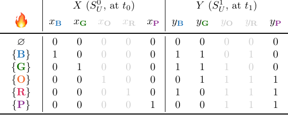
I will give a high-level overview and intuition of what gismo does and how it works, using the hotel smoke detector example problem describe above. For simplicity and brevity, let us assume $k = 1$. We now have the following truth table for $F_1 (X,Y)$:

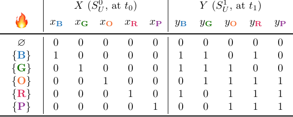
Gismo is initialised with candidate independent support $\mathcal{I} := \mathcal{G} = \{G_v := \{x_v, y_v\} \mid v \in V\}$. Hence, the corresponding candidate independent support is $I := \bigcup_{v \in V} G_v$. Then, it iterates over the groups $G_v$ in the partition. For each group, it checks for each variable if that variable can be removed from $I$ such that $I$ remains an independent support of $F_k (X,Y)$. If both variables can be removed, then the group is removed from $\mathcal{I}$ and the algorithm moves on to test the next group. If at least one variable needs to be part of $I$ for $I$ to be an independent support of $F_k (X,Y)$, then the group remains an element of $\mathcal{I}$ and is never considered again.

As an example, suppose that gismo starts with group $G_R$, and first tests if $y_R$ can be removed from $I$:

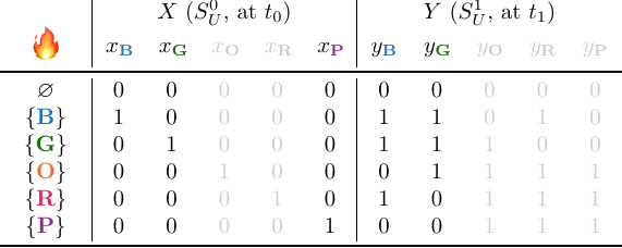
A quick inspection of the truth table above tells us that this is fine. All projected solutions are unique, none of them overlap. Gismo then checks if $x_{\textbf{R}}$ can also be removed from $I$. It turns out that it can, so gismo removes $G_{\textbf{R}}$ from $\mathcal{I}$ and moves on to the next group.

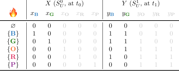
Suppose the next group is $G_{\textbf{O}}$. A quick inspection of the table shows that both $x_O$ and $y_O$ can be removed from $I$, and hence gismo also removes $G_{\textbf{O}}$ from $\mathcal{I}$, such that what we have left is $\mathcal{I} = {G_{\textbf{B}}, G_{\textbf{G}}, G_{\textbf{P}}}$:

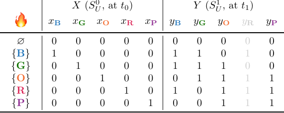
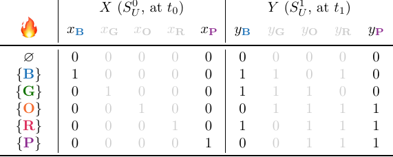
Suppose that gismo now decides to process group $G_P$, starting with variable $y_{\textbf{P}}$:

This is still fine, but as soon as gismo tries to remove $x_{\textbf{P}}$, something is wrong:

Specifically, we now see that the solutions for $\varnothing$ and $\{\textbf{P}\}$ overlap! Hence, gismo concludes that $G_{\textbf{P}}$ must be part of the GIS, and does not remove it from $\mathcal{I}$, but processes the next variable group.

Eventually, gismo finds that $\mathcal{I} := \{G_{\textbf{B}}, G_{\textbf{P}}\}$ is a GIS of $\langle F_1(X,Y), \mathcal{G}\rangle$, and returns. The resulting projected solutions are the following:

Notice how all the projected solutions are unique, and notice how they directly encode the signatures that we found for $k = 1$ and $D := \{\textbf{B}, \textbf{P}\}$ in the example problem at the beginning of this post.

Discussion

A key element of gismo is checking if a candidate GIS is indeed a GIS. Following the existing literature on independent supports, we do this by using Padoa’s Theorem (Padoa, 1901). Modulo a lot of details, the way to test if a variable should be part of the independent support is to construct a Boolean formula and check if it is unsatisfiable. If it is unsatisfiable, then the variable must be part of the independent support.

Hence, gismo makes at most $2 \cdot | V |$ SAT calls during its execution. We can think of these SAT calls as calls to a co-NP oracle. Consequently, testing if a candidate GIS is indeed a GIS, is computationally more expensive than checking if a candidate GICS is indeed a GICS, since that is polynomial in the size of the encoding (which in itself can be exponential in $k$, as discussed above).

You may also have noticed that, in the current implementation, gismo is a greedy algorithm. Hence, it can only guarantee a subset-minimal GIS.⁶ However, the ILP method for solving GICS as described in the literature guarantees a cardinality-minimal solution. Hence, it is possible that gismo returns a solution with a larger cardinality than the solution returned by the ILP method.

However, there is no good reason why we couldn’t create an implementation of gismo with the same guarantees as given by the former state of the art, other than that we just couldn’t be bothered. Feel free to contact us if you’re bored and want to give it a shot!

Also: we couldn’t be bothered to implement any optimisations. In fact gismo processes the groups in lexicographical order. This is not how you would do it if you wanted gismo to be fast, and this is not how you would do it if you wanted gismo to return a solution with a cardinality that is as small as possible. There are plenty of heuristics that can be used for a speedier execution of the algorithm and a smaller returned solution⁷, but we just never adapted them to the grouped setting. Again: if you’re bored, feel free to fork our repository and implement some of those heuristics!

Results

Our results can probably be summarised best in the following figure:

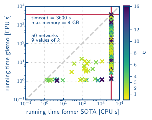
This scatter plot shows the running times of the entire encode+solve pipelines for our GIS-based pipeline (vertical axis), compared to the ILP-based pipeline that is based on the former state of the art (SOTA) (based on Padhee, Biswas, Pal, Basu and Sen, 2020), in CPU seconds, for 50 different networks and 9 different values of $k$ (indicated by colour). The network sizes vary from 10 to over 1 million nodes, and 14 to 1.5 million edges, with median degrees varying from 1 to 78. They are real-world networks sourced from the Network Repository (Rossi and Ahmed, 2015), and include networks of different types, like social networks and road networks. Any data point below the diagonal indicates that our gismo method solved that (network, $k$) combination faster than the former state of the art. Note that the axes are in log scale. We used a timeout time of 1 hour (3600 seconds), and allowed 4 GB of RAM.

In the above figure, we see that many of the instances ran out of either time or space. The largest instance that could be encoded to CNF using our method, had 227 320 nodes. On the other hand, the largest network that could be encoded into ILP by the former SATO, had 494 nodes. Hence, our method could encode networks that were 460$\times$ larger than the largest network that could be encoded by the state of the art.

The ILP method could also solve that instance within the permitted time (even though it could only encode it for $k=1$). The largest instance solved by our method had 21 363 nodes, and it could be solved for all tested values of $k$. This is a 43$\times$ improvement upon the former state of the art.

All instances that could be solved by the ILP method, could also be solved by our gismo-based method. For those instances that could be solved by both methods, we compared the cardinalities of the returned solutions. We found that for the majority of those instances, the cardinality of the solution computed by the gismo-based method was either equal to, or at most 10% larger than the cardinality of the solution returned by the ILP-based method.

Recall that we made zero efforts to optimise gismo to make it fast or return a small solution, so we think that there is still a lot of room for improvement of these results here. On the other hand, we spent quite some time trying to improve the ILP-based method, managing to increase the size of the largest network it could handle from ~300 nodes to ~500 nodes. However, we always ended up paying either in terms of memory use, or in terms of running time. You can find a link to the extended version of our paper with more details on this here.

Take-aways

In this work, we demonstrated how we can solve larger problems instances and solve them faster, by reducing the original problem to a computationally harder problem, and developing a solver that was fast and good enough in practice to be of practical use.

Note that this is possible because today’s SAT solvers are so incredibly fast at solving NP-hard problems. This opens the door for us to start working on developing practical tools that solve problems that are higher up the polynomial hierarchy, meaning that we can start to model and solve problems that are higher up the polynomial hierarchy.

Exciting times!

Footnotes